Cloud backtesting: when CPUs, GPUs and parallel runs pay off
Buy a faster answer to a defined question. More hardware and more parameter combinations are different purchases.
Research cutoff: 22 October 2026. Evidence synthesis and original analytical frameworks; no platform performance experiment.

The key distinction
Compare complete workloads using wall time, total cost and valid results. GPUs and parallel execution help only when the algorithm and data path can use them; a larger search does not make its selected strategy more credible.
Start with the decision you need sooner
Which cloud machine should run a trading backtest? Start by identifying the work that delays a research decision, then measure whether a different resource reduces that delay at an acceptable total cost. CPU count, GPU count and advertised hourly price do not answer that question independently.
This article supplies an engineering decision framework and transparent mathematical scenarios. It does not present a measured VC Trader AI benchmark, a cloud price comparison or a trading strategy experiment. The distinction matters: a theoretical scaling limit can prevent a poor purchase, but cannot establish the fastest implementation of your code.
Define one reference task before selecting hardware: a fixed dataset, strategy version, cost model, candidate set and required outputs. If the faster run omits transaction costs or processes fewer observations, it has not demonstrated a speed improvement for the same task.
Profile the whole route from data to result
Separate data access, decoding, feature construction, simulation, aggregation and artifact writing. Measure wall time and peak memory around each stage, including setup and queues. Record whether the data were cached. A warm local file and a cold remote download are different operating conditions.
Parallel scaling depends on the algorithm, application, communication and memory behaviour. LLNL’s tutorial explains these dependencies and overheads. Hardware alone does not make a workload parallel. [1]
| Observed bottleneck | Candidate intervention | Required check |
|---|---|---|
| Repeated file reads | Reuse parsed data; improve layout | Cold and warm timings, storage cost |
| One sequential simulation | Optimise hot loop or algorithm | Same fills and state transitions |
| Independent runs | Parallel jobs with bounded concurrency | Aggregate throughput and complete outcomes |
| Compatible dense array work | Consider GPU implementation | Transfer overhead, precision and memory |
| Results too large to hold | Partition or stream data | Boundary effects and aggregation correctness |
A GPU allocation is not a GPU implementation
A simulation may branch on each event and update path-dependent state. Another workload may apply the same numerical operation across a large array. Those structures suggest different experiments with acceleration. Do not infer that every Python backtest maps efficiently to a GPU because machine-learning training often does.
AWS Batch documents GPU resource requests and reserves those devices for a job’s duration. It also warns that jobs which do not use a GPU can still run on GPU instances and may cost more than comparable non-GPU resources. Resource allocation is a scheduling feature, not evidence of acceleration. [2]
For a candidate GPU port, first compare output equivalence. Record dtype, tolerances and whether calculations changed order. Then time data transfer, initialisation and computation together. Report datasets for which the GPU loses as well as those for which it wins. Without that boundary, a benchmark can describe a favourable case while concealing its operating conditions.
Parallel runs and faster individual runs are different
A parameter sweep can distribute separate simulations even if each one remains sequential. AWS Batch array jobs support related independent jobs, potentially running concurrently across hosts. The documentation cites parameter sweeps and Monte Carlo work as examples. That establishes scheduling capability, not a guaranteed runtime reduction. [3]
Ask whether the goal is latency or throughput. A researcher waiting for one final validation cares about time to that result. A batch exploring independent candidates may care about completed valid runs per hour. The same configuration can improve throughput while leaving the slowest individual run unchanged.
Bound concurrency before launch. Make data versions immutable, assign distinct output paths and record every attempt. A worker that retries a failed simulation should not overwrite evidence of the original failure. Queue saturation, shared storage and duplicated loading can turn nominal parallelism into a slower pipeline.
A transparent speedup calculation
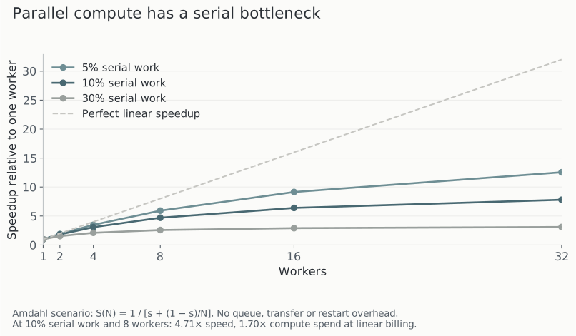
For an ideal fixed workload, Amdahl’s model gives speedup S(N) = 1 / (s + (1 − s) / N), where s is the serial share of single-worker time and N is the number of ideal identical workers. Cornell’s tutorial also distinguishes this fixed-work question from increasing the problem size as resources grow. [4]
In our explicitly hypothetical scenario, s = 0.10 and N = 8 produce S = 4.71, rounded. Even infinitely many ideal workers cannot exceed 10 times speedup with that unchanged serial fraction. These figures are arithmetic consequences of the assumptions, not observations of trading software.
If all eight workers are billed for the entire run at an identical per-worker rate, compute cost relative to one worker is N / S, or 1.70 in this scenario. That model excludes startup, storage, network charges, discounts and different instance designs. It illustrates why reducing elapsed time can increase total compute spend. Substitute measured timings before using the model for procurement.
Compare the cost of an accepted research result
AWS states that Batch has no additional service charge while underlying resources are billed. A free scheduler is therefore compatible with a costly workload. No regional resource prices are quoted here because a reproducible comparison needs a dated configuration and billing basis. [5]
Our accounting proposal is: total experiment cost equals compute plus storage, transfer, orchestration services, paid data or inference, and attributable recovery effort. Define accepted output before the run. Then divide total batch cost by the number of outputs that satisfy the predeclared technical checks. Keep economic strategy performance separate from computational validity.
For a simple break-even comparison, a faster configuration must save enough runtime to offset its rate premium and incremental overhead. With rates r expressed in currency per hour, runtime t in hours and other costs o in the same currency, compare r_A * t_A + o_A against r_B * t_B + o_B. State currency, region, tax treatment, date, on-demand or discounted basis and whether idle provisioned time is included. Do not compare a discounted long-term commitment with an on-demand alternative without explaining the commitment risk.
More compute can increase the selection problem
Compute changes the opportunity to search. It does not remove the need to separate development from evaluation. If a new cluster explores many more variants, the resulting best historical strategy is the winner of a larger selection process. Its headline improvement is not automatically stronger evidence.
Reserve evaluation data and freeze the selection procedure before expanding the search. Record failed configurations and abandoned experiments. A decision to stop searching after a promising result is also part of the procedure. Read the walk-forward and overfitting guide for chronological validity and repeated selection.
There is a legitimate counter-case: extra compute can make better checks affordable, including sensitivity analyses, more realistic fills and broader stress scenarios. The value depends on what the additional computation buys. Spend that budget on disconfirmation as deliberately as on finding a better equity curve.
A benchmark protocol a buyer can reuse
- Freeze the task, dataset provenance, environment, versions, seeds and output checks.
- State machine specifications, region, concurrency, cache state and billing assumptions.
- Measure setup, queue, compute and export times separately, then report end-to-end wall time.
- Repeat enough to expose relevant variability; publish the repeat count, individual results and failures.
- Compare output equivalence before comparing speed, then calculate complete cost per accepted result.
- Document the operating boundary: dataset size, workload type and conditions under which the alternative loses.
VC Trader AI’s public scope includes Python research, cloud backtesting and managed deployment. This guide makes no measured claim about its speed or cost. Research compute and a continuously hosted live strategy also have different availability requirements; see the Python-to-MT5 handoff before treating a research job as an execution service.
The purchase decision should follow the experiment: use the least costly configuration that produces a timely, inspectable answer to the question you actually froze. Revisit it when the workload changes.
Sources and scope
- [1] Blaise Barney and Donald Frederick, Lawrence Livermore National Laboratory: Introduction to Parallel Computing Tutorial
- [2] Amazon Web Services: Run GPU jobs
- [3] Amazon Web Services: Array jobs
- [4] Cornell Center for Advanced Computing: Amdahl’s Law
- [5] Amazon Web Services: AWS Batch pricing
Sources checked on 22 October 2026. Organisational authorship: Vanquish Capital Technologies, with AI assistance. External findings, proposed engineering criteria and mathematical scenarios are distinguished in the text. Product statements describe the current first-party early-access scope, not independent verification of every control. No customer outcome, original trading experiment or investment recommendation is claimed.